Reasons for modifying the data

Sometimes you need to do stuff to your data before you can use it. Moreover, you’re often dealing with data that’s split into train/test sets. In this case you need to work out what to do with your data based solely on the training set and then apply that—without changing your method—to the test set. If you’re dealing with \(K\)-fold cross-validation, then you’ve got \(K\) training sets and \(K\) test sets, and so you need to repeat this \(K\) times.

A good example is missing value imputation, where you have some missing data in your train/test sets and you need to fill them in via some imputation method. I’m no expert on the topic (but I hope to be after the missing value imputation tutorial tomorrow!) but I’ve seen this done wrong before in StackExchange answers and in Kaggle solutions: the imputation is done before the data is split into train/test. This is called data leakage, and models assessed using the test set will appear more accurate than they are, because they’ve already had a sneak preview of the data.

So the mindset is clear: don’t touch the test set until the last possible moment. The recipes package follows this mindset. First you create a recipe, which is a blueprint for how you will process your data. At this point, no data has been modified. Then you prep the recipe using your training set, which is where the actual processing is defined and all the parameters worked out. Finally, you can bake the training set, test set, or any other data set with similar columns, and in this step the actual modification takes place.

Missing value imputation isn’t the only reason to process data, though. Processing can involve:

• Centering and scaling the predictors. Some models (K-NN, SBMs, PLS, neural networks) require that the predictor variables have the same units.
• Applying filters or PCA signal extraction to deal with correlation between predictors.
• Encoding data, such as turning factors into Boolean dummy variables, or turning dates into days of the week.
• Developing new features (ie. feature engineering).

The ames data

We load the data with the make_ames function from the AmesHousing package.

ames <- AmesHousing::make_ames()
ames %>% str

## Classes 'tbl_df', 'tbl' and 'data.frame':    2930 obs. of  81 variables:
##  $ MS_SubClass       : Factor w/ 16 levels "One_Story_1946_and_Newer_All_Styles",..: 1 1 1 1 6 6 12 12 12 6 ...
##  $ MS_Zoning         : Factor w/ 7 levels "Floating_Village_Residential",..: 3 2 3 3 3 3 3 3 3 3 ...
##  $ Lot_Frontage      : num  141 80 81 93 74 78 41 43 39 60 ...
##  $ Lot_Area          : int  31770 11622 14267 11160 13830 9978 4920 5005 5389 7500 ...
##  $ Street            : Factor w/ 2 levels "Grvl","Pave": 2 2 2 2 2 2 2 2 2 2 ...
##  $ Alley             : Factor w/ 3 levels "Gravel","No_Alley_Access",..: 2 2 2 2 2 2 2 2 2 2 ...
##  $ Lot_Shape         : Factor w/ 4 levels "Regular","Slightly_Irregular",..: 2 1 2 1 2 2 1 2 2 1 ...
##  $ Land_Contour      : Factor w/ 4 levels "Bnk","HLS","Low",..: 4 4 4 4 4 4 4 2 4 4 ...
##  $ Utilities         : Factor w/ 3 levels "AllPub","NoSeWa",..: 1 1 1 1 1 1 1 1 1 1 ...
##  $ Lot_Config        : Factor w/ 5 levels "Corner","CulDSac",..: 1 5 1 1 5 5 5 5 5 5 ...
##  $ Land_Slope        : Factor w/ 3 levels "Gtl","Mod","Sev": 1 1 1 1 1 1 1 1 1 1 ...
##  $ Neighborhood      : Factor w/ 28 levels "North_Ames","College_Creek",..: 1 1 1 1 7 7 17 17 17 7 ...
##  $ Condition_1       : Factor w/ 9 levels "Artery","Feedr",..: 3 2 3 3 3 3 3 3 3 3 ...
##  $ Condition_2       : Factor w/ 8 levels "Artery","Feedr",..: 3 3 3 3 3 3 3 3 3 3 ...
##  $ Bldg_Type         : Factor w/ 5 levels "OneFam","TwoFmCon",..: 1 1 1 1 1 1 5 5 5 1 ...
##  $ House_Style       : Factor w/ 8 levels "One_and_Half_Fin",..: 3 3 3 3 8 8 3 3 3 8 ...
##  $ Overall_Qual      : Factor w/ 10 levels "Very_Poor","Poor",..: 6 5 6 7 5 6 8 8 8 7 ...
##  $ Overall_Cond      : Factor w/ 10 levels "Very_Poor","Poor",..: 5 6 6 5 5 6 5 5 5 5 ...
##  $ Year_Built        : int  1960 1961 1958 1968 1997 1998 2001 1992 1995 1999 ...
##  $ Year_Remod_Add    : int  1960 1961 1958 1968 1998 1998 2001 1992 1996 1999 ...
##  $ Roof_Style        : Factor w/ 6 levels "Flat","Gable",..: 4 2 4 4 2 2 2 2 2 2 ...
##  $ Roof_Matl         : Factor w/ 8 levels "ClyTile","CompShg",..: 2 2 2 2 2 2 2 2 2 2 ...
##  $ Exterior_1st      : Factor w/ 16 levels "AsbShng","AsphShn",..: 4 14 15 4 14 14 6 7 6 14 ...
##  $ Exterior_2nd      : Factor w/ 17 levels "AsbShng","AsphShn",..: 11 15 16 4 15 15 6 7 6 15 ...
##  $ Mas_Vnr_Type      : Factor w/ 5 levels "BrkCmn","BrkFace",..: 5 4 2 4 4 2 4 4 4 4 ...
##  $ Mas_Vnr_Area      : num  112 0 108 0 0 20 0 0 0 0 ...
##  $ Exter_Qual        : Factor w/ 4 levels "Excellent","Fair",..: 4 4 4 3 4 4 3 3 3 4 ...
##  $ Exter_Cond        : Factor w/ 5 levels "Excellent","Fair",..: 5 5 5 5 5 5 5 5 5 5 ...
##  $ Foundation        : Factor w/ 6 levels "BrkTil","CBlock",..: 2 2 2 2 3 3 3 3 3 3 ...
##  $ Bsmt_Qual         : Factor w/ 6 levels "Excellent","Fair",..: 6 6 6 6 3 6 3 3 3 6 ...
##  $ Bsmt_Cond         : Factor w/ 6 levels "Excellent","Fair",..: 3 6 6 6 6 6 6 6 6 6 ...
##  $ Bsmt_Exposure     : Factor w/ 5 levels "Av","Gd","Mn",..: 2 4 4 4 4 4 3 4 4 4 ...
##  $ BsmtFin_Type_1    : Factor w/ 7 levels "ALQ","BLQ","GLQ",..: 2 6 1 1 3 3 3 1 3 7 ...
##  $ BsmtFin_SF_1      : num  2 6 1 1 3 3 3 1 3 7 ...
##  $ BsmtFin_Type_2    : Factor w/ 7 levels "ALQ","BLQ","GLQ",..: 7 4 7 7 7 7 7 7 7 7 ...
##  $ BsmtFin_SF_2      : num  0 144 0 0 0 0 0 0 0 0 ...
##  $ Bsmt_Unf_SF       : num  441 270 406 1045 137 ...
##  $ Total_Bsmt_SF     : num  1080 882 1329 2110 928 ...
##  $ Heating           : Factor w/ 6 levels "Floor","GasA",..: 2 2 2 2 2 2 2 2 2 2 ...
##  $ Heating_QC        : Factor w/ 5 levels "Excellent","Fair",..: 2 5 5 1 3 1 1 1 1 3 ...
##  $ Central_Air       : Factor w/ 2 levels "N","Y": 2 2 2 2 2 2 2 2 2 2 ...
##  $ Electrical        : Factor w/ 6 levels "FuseA","FuseF",..: 5 5 5 5 5 5 5 5 5 5 ...
##  $ First_Flr_SF      : int  1656 896 1329 2110 928 926 1338 1280 1616 1028 ...
##  $ Second_Flr_SF     : int  0 0 0 0 701 678 0 0 0 776 ...
##  $ Low_Qual_Fin_SF   : int  0 0 0 0 0 0 0 0 0 0 ...
##  $ Gr_Liv_Area       : int  1656 896 1329 2110 1629 1604 1338 1280 1616 1804 ...
##  $ Bsmt_Full_Bath    : num  1 0 0 1 0 0 1 0 1 0 ...
##  $ Bsmt_Half_Bath    : num  0 0 0 0 0 0 0 0 0 0 ...
##  $ Full_Bath         : int  1 1 1 2 2 2 2 2 2 2 ...
##  $ Half_Bath         : int  0 0 1 1 1 1 0 0 0 1 ...
##  $ Bedroom_AbvGr     : int  3 2 3 3 3 3 2 2 2 3 ...
##  $ Kitchen_AbvGr     : int  1 1 1 1 1 1 1 1 1 1 ...
##  $ Kitchen_Qual      : Factor w/ 5 levels "Excellent","Fair",..: 5 5 3 1 5 3 3 3 3 3 ...
##  $ TotRms_AbvGrd     : int  7 5 6 8 6 7 6 5 5 7 ...
##  $ Functional        : Factor w/ 8 levels "Maj1","Maj2",..: 8 8 8 8 8 8 8 8 8 8 ...
##  $ Fireplaces        : int  2 0 0 2 1 1 0 0 1 1 ...
##  $ Fireplace_Qu      : Factor w/ 6 levels "Excellent","Fair",..: 3 4 4 6 6 3 4 4 6 6 ...
##  $ Garage_Type       : Factor w/ 7 levels "Attchd","Basment",..: 1 1 1 1 1 1 1 1 1 1 ...
##  $ Garage_Finish     : Factor w/ 4 levels "Fin","No_Garage",..: 1 4 4 1 1 1 1 3 3 1 ...
##  $ Garage_Cars       : num  2 1 1 2 2 2 2 2 2 2 ...
##  $ Garage_Area       : num  528 730 312 522 482 470 582 506 608 442 ...
##  $ Garage_Qual       : Factor w/ 6 levels "Excellent","Fair",..: 6 6 6 6 6 6 6 6 6 6 ...
##  $ Garage_Cond       : Factor w/ 6 levels "Excellent","Fair",..: 6 6 6 6 6 6 6 6 6 6 ...
##  $ Paved_Drive       : Factor w/ 3 levels "Dirt_Gravel",..: 2 3 3 3 3 3 3 3 3 3 ...
##  $ Wood_Deck_SF      : int  210 140 393 0 212 360 0 0 237 140 ...
##  $ Open_Porch_SF     : int  62 0 36 0 34 36 0 82 152 60 ...
##  $ Enclosed_Porch    : int  0 0 0 0 0 0 170 0 0 0 ...
##  $ Three_season_porch: int  0 0 0 0 0 0 0 0 0 0 ...
##  $ Screen_Porch      : int  0 120 0 0 0 0 0 144 0 0 ...
##  $ Pool_Area         : int  0 0 0 0 0 0 0 0 0 0 ...
##  $ Pool_QC           : Factor w/ 5 levels "Excellent","Fair",..: 4 4 4 4 4 4 4 4 4 4 ...
##  $ Fence             : Factor w/ 5 levels "Good_Privacy",..: 5 3 5 5 3 5 5 5 5 5 ...
##  $ Misc_Feature      : Factor w/ 6 levels "Elev","Gar2",..: 3 3 2 3 3 3 3 3 3 3 ...
##  $ Misc_Val          : int  0 0 12500 0 0 0 0 0 0 0 ...
##  $ Mo_Sold           : int  5 6 6 4 3 6 4 1 3 6 ...
##  $ Year_Sold         : int  2010 2010 2010 2010 2010 2010 2010 2010 2010 2010 ...
##  $ Sale_Type         : Factor w/ 10 levels "COD","Con","ConLD",..: 10 10 10 10 10 10 10 10 10 10 ...
##  $ Sale_Condition    : Factor w/ 6 levels "Abnorml","AdjLand",..: 5 5 5 5 5 5 5 5 5 5 ...
##  $ Sale_Price        : int  215000 105000 172000 244000 189900 195500 213500 191500 236500 189000 ...
##  $ Longitude         : num  -93.6 -93.6 -93.6 -93.6 -93.6 ...
##  $ Latitude          : num  42.1 42.1 42.1 42.1 42.1 ...

Now we will split the data into test and train. We’ll reserve 25% of of the data for testing.

library(rsample)
set.seed(4595)
data_split <- initial_split(ames, strata = "Sale_Price", p = 0.75)
ames_train <- training(data_split)
ames_test <- testing(data_split)

A simple log-transform

The first of Max’s examples is a really simple log transform of Sale_Price. Suppose we use the formula log10(Sale_Price) ~ Longitude + Latitude. The steps are:

1. Assign Sale_Price to the outcome.
2. Assign Longitude and Latittude as predictors.
3. Log transform the outcome.

The way to define this in recipes is as follows:

mod_rec <- recipe(Sale_Price ~ Longitude + Latitude, data = ames_train) %>% 
    step_log(Sale_Price, base = 10)

Infrequently occurring levels

We usually encode factors as Boolean dummy variables, with R often taking care of this in the background. If there are C levels of the factor, only C - 1 dummy variables are required. But what if you have very few values for a particular level? For example, the Neighborhood predictor in our ames data:

ames %>% 
    ggplot(aes(x = Neighborhood)) +
    geom_bar(fill = "#6d1e3b", colour = "white") + # I don't like the default grey
    coord_flip()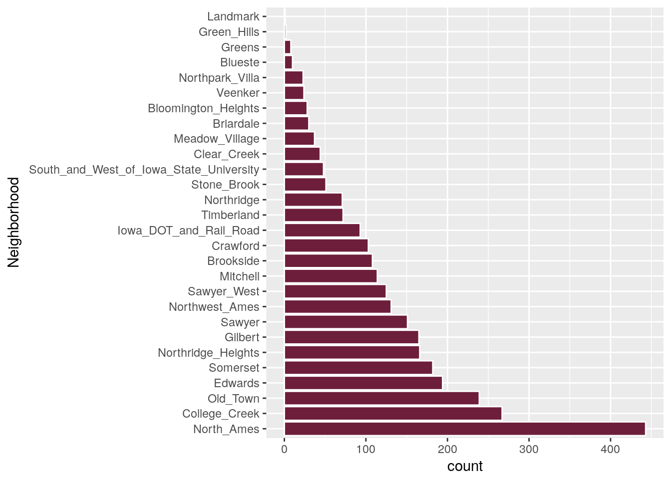

In fact, there’s only one data point with a Neighborhood of Landmark. This is called a “zero-variance predictor”. There are two main approaches here:

1. remove any data points with infrequently occurring values, or
2. group all of the infrequently occurring values into an “Other” level.

This is a job for the recipes package, and Max takes us through the example.

We can take care of the infrequently occurring levels here using the step_other function. In this case, we “other” any level that occurs fewer than 5% of the time. We can then create dummy variables for all factor variables with step_dummy:

mod_rec <- recipe(Sale_Price ~ Longitude + Latitude + Neighborhood, 
                  data = ames_train) %>% 
    step_log(Sale_Price, base = 10) %>% # The log-transform from earlier
    step_other(Neighborhood, threshold = 0.05) %>%
    step_dummy(all_nominal())

The recipes process

Recipes work in a three-step process: recipe –> prepare –> bake/juice. We can think of this as: define –> estimate –> apply. juice only applies to the original data set defined in the recipe, the idea at the core of bake is that it can be applied to an arbitrary data set.

First we prep the data using the recipe in Max’s example:

mod_rec_trained <- mod_rec %>% 
    prep(training = ames_train, retain = TRUE)
mod_rec_trained

## Data Recipe
## 
## Inputs:
## 
##       role #variables
##    outcome          1
##  predictor          3
## 
## Training data contained 2199 data points and no missing data.
## 
## Operations:
## 
## Log transformation on Sale_Price [trained]
## Collapsing factor levels for Neighborhood [trained]
## Dummy variables from Neighborhood [trained]

We can now bake the recipe, applying it to the test set we defined earlier:

ames_test_dummies <- mod_rec_trained %>% bake(newdata = ames_test)
names(ames_test_dummies)

##  [1] "Sale_Price"                      "Longitude"                      
##  [3] "Latitude"                        "Neighborhood_College_Creek"     
##  [5] "Neighborhood_Old_Town"           "Neighborhood_Edwards"           
##  [7] "Neighborhood_Somerset"           "Neighborhood_Northridge_Heights"
##  [9] "Neighborhood_Gilbert"            "Neighborhood_Sawyer"            
## [11] "Neighborhood_other"

Other uses

I have to admit that the rest got away from me a little bit, because I’m not overly familiar with all of the transformations/methods that were used (what is a Yeo-Johnson Power Transformation?!).

However, there’s a tonne of cool stuff in the slides that I’ll be coming back to later, I’m sure. Max used recipes and rsample to:

• deal with interactions between predictors,
• apply processing to all of the folds of a 10-fold cross-validation,
• train 10 linear models on that same 10-fold cross-validation,
• assess and plot the performance of those linear models, and
• train and asses 10 nearest-neighbour models on the 10-fold cross-validation.

I know I’ll be using this recipes package a lot.